1. Simple metadynamics simulation guide

2. 集合变量配位数函数

3. Biochemical systems metadynamics 

4. 自由能面绘图软件graph.sopt

5. cp2k和plumed联用简单案例

6. Tree diagram of keywords ralated to metadynamics

7. CP2K元动力学中获取重构势能面的方法

8. 基于restart文件继续执行元动力学

9. 元动力学测试题

Metadynamics is a computational method used in molecular simulations to enhance the sampling of free energy landscapes by adding a bias potential. It was developed to overcome the problem of slow conformational transitions and improve the exploration of rare events in complex systems.

Metadynamics was first introduced in 2002 by Michele Parrinello and Alessandro Laio. It builds upon previous methods such as umbrella sampling and adaptive biasing force, and is based on the idea of filling free energy basins with Gaussian hills to encourage the system to explore new areas of the configuration space.

Metadynamics allows researchers to study complex phenomena such as protein folding, protein-ligand binding, and phase transitions. It has also been applied to study chemical reactions and material properties. By enhancing the sampling of free energy landscapes, metadynamics enables the calculation of kinetic and thermodynamic properties that would be difficult to obtain otherwise.

In metadynamics, the external history-dependent bias potential is a function that is added to the potential energy of the system in order to drive it towards regions of phase space that have not been explored yet. The bias potential depends on the collective variables (CVs), which are coordinates that describe the system and are used to monitor its progress in exploring phase space. The bias potential is constructed so that it grows with time in regions of phase space that have not been visited frequently, effectively creating a "hill" in the potential energy landscape that drives the system towards unexplored regions. This results in an increased exploration of the phase space and the generation of a smooth free energy surface that describes the system's behavior. The external history-dependent bias potential is what makes metadynamics a powerful technique for exploring complex, high-dimensional systems.

The external history-dependent bias potential in metadynamics can be expressed by the following equation:

V_bias(s) = ∑ w_i exp(-||s-s_i||^2/2σ^2)

where V_bias is the bias potential, s is a vector of collective variables that describe the system, w_i is the height of the Gaussian hills added to the potential energy landscape, s_i is the position of the ith Gaussian hill in collective variable space, and σ is the width of the Gaussians. The summation is taken over all previous time steps of the simulation. The idea is to add up a series of Gaussians at previously visited regions of the collective variable space, effectively creating a repulsive bias that pushes the system away from those regions and towards unexplored regions. As a result, the system is encouraged to explore a larger portion of the phase space, which can lead to more accurate free energy calculations and a better understanding of the system's behavior.

CP2K can perform metadynamics simulations, which are a type of free energy calculation that use a history-dependent bias potential to explore the energy landscape of a system. You can set up a metadynamics calculation by adding the section MOTION / FREE_ENERGY / METADYN in your CP2K input file. In this section, you can specify the collective variables (CVs) on which to apply metadynamics, the frequency and height of the Gaussian hills, the friction term and the temperature for the extended Lagrangian scheme, and other options. You can also monitor the behavior of the CVs and the bias potential during the simulation.

1. Simple metadynamics simulation guide

Metadynamics is a powerful enhanced sampling technique that can be used to investigate complex systems, including those with multiple degrees of freedom. In metadynamics, a history-dependent bias is added to the potential energy of the system, which drives the system towards regions of high free energy and enhances the exploration of the configuration space.

One possible implementation of metadynamics using the coordination numbers as variables could be as follows:

1. Define the coordinates of the system: In this case, the coordination numbers can be used as collective variables (CVs) to represent the system. The coordination numbers could be calculated based on the distances between the atoms in the system and their neighbors.

2. Choose the Gaussian height and width: The height and width of the Gaussian hills used in the bias potential should be carefully chosen to achieve a good balance between exploration and convergence. A common choice is to use a height of 0.1-1.0 kJ/mol and a width of 0.1-0.5 Å.

3. Initialize the simulation: Start the simulation from an initial configuration and run it for a certain amount of time without the metadynamics bias. This allows the system to equilibrate and reach its initial state.

4. Add the metadynamics bias: At regular intervals (e.g., every 500-1000 time steps), add a Gaussian hill centered at the current value of the CVs to the potential energy of the system. Repeat this process until the simulation has run for a sufficient amount of time to generate a good sampling of the configuration space.

5. Analyze the results: The final state of the simulation can be analyzed to gain insights into the thermodynamics and kinetics of the system. The distribution of the CVs can be plotted and used to identify free energy basins and transition states.

This is a simple example of how metadynamics can be implemented using coordination numbers as variables, but many other variations and modifications are possible, depending on the specifics of the system being studied.

The important keywords related to metadynamics in CP2K.

METADYN	This section sets parameters to set up a calculation of metadynamics.
METAVAR	This section specify the nature of the collective variables.
FREE_ENERGY	Controls the calculation of free energy and free energy derivatives with different possible methods
FREE_ENERGY/METHOD	Defines the method to use to compute free energy.  Default value: METADYN
DO_HILLS	This keyword enables the spawning of the hills. Default .FALSE
NT_HILLS	Specify the maximum MD step interval between spawning two hills.  Default value: 30
WW	Specifies the height of the gaussian to spawn. Default 0.1
SCALE	Specifies the scale factor for the following collective variable. Alias names for this keyword: WIDTH
METAVAR/COLVAR	Specifies the colvar on which to apply metadynamics.
METADYN/PRINT	Controls the printing properties during an metadynamics run
METADYN/PRINT/COLVAR	Controls the printing of COLVAR summary information during metadynamics. When an extended Lagrangian use used, the files contain (in order): colvar value of the extended Lagrangian, instantaneous colvar value, force due to the harmonic term of the extended Lagrangian and the force due to the previously spawned hills, the force due to the walls, the velocities in the extended Lagrangian, the potential of the harmonic term of the Lagrangian, the potential energy of the hills, the potential energy of the walls and the temperature of the extended Lagrangian. When the extended Lagrangian is not used, all related fields are omitted.
COMMON_ITERATION_LEVELS	How many iterations levels should be written in the same file (no extra information about the actual iteration level is written to the file) Default value: 0
METADYN/PRINT/HILLS	Controls the printing of HILLS summary information during metadynamics. The file contains: instantaneous colvar value, width of the spawned gaussian and height of the gaussian. According the value of the EACH keyword this file may not be synchronized with the COLVAR file.  也就是说如果只有一个集合变量的话，输出的HILLS.metadynLog文件中会存在4列，第一列为时间，第二列为相应时刻添加gaussian hill时集合变量瞬时值，第三列为添加的gasuuian hill的宽度，对应SCALE关键词数值，第四列是添加的gaussian hill的高度，对应设WW关键词数值，该值默认为0.1。
MOTION / PRINT / RESTART	Controls the dumping of the restart file during runs. By default keeps a short history of three restarts. See also RESTART_HISTORY
MOTION / PRINT / RESTART_HISTORY	Dumps unique restart files during the run keeping all of them.Most useful if recovery is needed at a later point.
FORCE_EVAL / SUBSYS / COLVAR	This section specifies the nature of the collective variables.
SUBSYS / COLVAR / COORDINATION	Section to define the coordination number as a collective variable.
KINDS_FROM	Specify alternatively kinds of atoms building the coordination variable.
KINDS_TO	Specify alternatively kinds of atoms building the coordination variable.
R0	Specify the R0 parameter in the coordination function。 Default value: 3.00000000E+000 Default unit: [bohr] Alias names for this keyword: R_0
NN	Sets the value of the numerator of the exponential factorin the coordination FUNCTION. Default value: 6 Alias names for this keyword: EXPON_NUMERATOR
ND	Sets the value of the denominator of the exponential factorin the coordination FUNCTION. Default value: 12 Alias names for this keyword: EXPON_DENOMINATOR

2. 集合变量配位数函数

 SUBSYS / COLVAR / COORDINATION 关键词的表达式

 以下是该方程的中文解释：

• N_coord(A, B) 表示集合 A 中的原子或粒子相对于集合 B 的配位数。
• N_A 表示集合 A 中的总原子或粒子数。
• N_B 表示集合 B 中的总原子或粒子数。
• r_ij 表示集合 B 中的原子或粒子 i 与集合 A 中的原子或粒子 j 之间的距离。
• d_AB 表示集合 A 和 B 之间的特征距离。
• p 和 q 是确定配位函数形状的参数。

该方程通过对集合 A 中的所有粒子求和来计算配位数 N_coord(A, B)。对于集合 A 中的每个粒子，该方程计算其对配位数的贡献，方法是对集合 B 中的所有粒子求和，其中每个粒子的贡献是其与集合 A 中的粒子的距离的函数。

用于计算集合 B 中每个粒子的贡献的函数是径向分布函数的修改版本，该函数测量在给定距离处找到粒子的概率。修改后的函数考虑了粒子的形状和它们相互作用的强度。参数 p 和 q 用于控制函数的形状和它的有效距离范围。

总的来说，该方程提供了一种量化集合 A 中的粒子与集合 B 中的粒子配位程度的方法，考虑了粒子的形状和相互作用的强度。

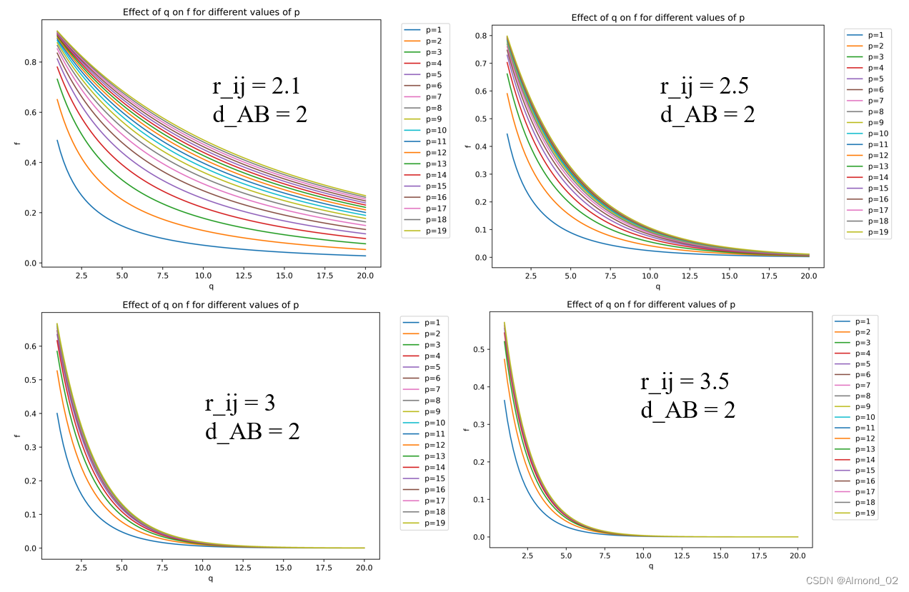
p和q同时对配位数的影响 

# -*- coding: utf-8 -*-
"""
Created on Thu Feb 23 12:45:37 2023@author: sun78
"""import numpy as npdef coordination_number(A, B, r, d_AB, p, q):# Calculate the distance matrix between atoms in A and BR = np.sqrt(np.sum((A[:, np.newaxis] - B) ** 2, axis=2))# Calculate the coordination number for each atom in AN_coord = np.zeros(len(A))for i in range(len(A)):r_ij = R[i]N_A = len(A)N_B = len(B)g = np.sum((1 - (r_ij / d_AB) ** p) / (1 - (r_ij / d_AB) ** (p + q)))N_coord[i] = (1 / N_A) * (1 / N_B) * greturn N_coordimport matplotlib.pyplot as plt# Define the coordinates of the atoms in set A and B
A = np.array([[0, 0, 0], [1, 1, 1], [2, 2, 2]])
B = np.array([[0, 1, 1], [1, 0, 1], [1, 1, 0], [2, 1, 1], [1, 2, 1], [1, 1, 2]])# Define the radii of the atoms in set B
r = np.array([1.0, 1.0, 1.0, 1.0, 1.0, 1.0])# Define the characteristic distance between sets A and B
d_AB = 2.5# Define the range of p and q values to plot
p_range = np.linspace(2, 10, 50)
q_range = np.linspace(2, 20, 50)# Calculate the coordination number for each p and q value
N_coord = np.zeros((len(p_range), len(q_range)))
for i, p in enumerate(p_range):for j, q in enumerate(q_range):N_coord[i, j] = np.mean(coordination_number(A, B, r, d_AB, p, q))# Plot the results
fig, ax = plt.subplots()
cax = ax.imshow(N_coord.T, extent=[p_range.min(), p_range.max(), q_range.min(), q_range.max()],origin='lower', cmap='viridis', aspect='auto')
ax.set_xlabel('p')
ax.set_ylabel('q')
cbar = fig.colorbar(cax)
cbar.set_label('Coordination Number')
plt.show()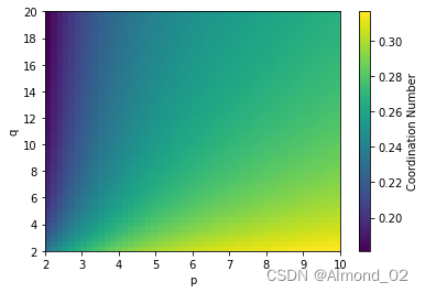

 d_AB对配位数的影响

import numpy as npdef coordination_number(A, B, r, d_AB, p, q):# Calculate the distance matrix between atoms in A and BR = np.sqrt(np.sum((A[:, np.newaxis] - B) ** 2, axis=2))# Calculate the coordination number for each atom in AN_coord = np.zeros(len(A))for i in range(len(A)):r_ij = R[i]N_A = len(A)N_B = len(B)g = np.sum((1 - (r_ij / d_AB) ** p) / (1 - (r_ij / d_AB) ** (p + q)))N_coord[i] = (1 / N_A) * (1 / N_B) * greturn N_coordimport matplotlib.pyplot as plt# Define the coordinates of the atoms in set A and B
A = np.array([[0, 0, 0], [1, 1, 1], [2, 2, 2]])
B = np.array([[0, 1, 1], [1, 0, 1], [1, 1, 0], [2, 1, 1], [1, 2, 1], [1, 1, 2]])# Define the radii of the atoms in set B
r = np.array([1.0, 1.0, 1.0, 1.0, 1.0, 1.0])# Define the values of p and q to use
p = 5
q = 10# Define the range of d_AB values to plot
d_AB_range = np.linspace(1, 5, 50)# Calculate the coordination number for each d_AB value
N_coord = np.zeros(len(d_AB_range))
for i, d_AB in enumerate(d_AB_range):N_coord[i] = np.mean(coordination_number(A, B, r, d_AB, p, q))# Plot the results
fig, ax = plt.subplots()
ax.plot(d_AB_range, N_coord)
ax.set_xlabel('d_AB')
ax.set_ylabel('Coordination Number')
plt.show()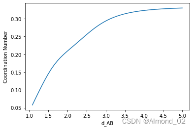

q值对配位数的影响 

import numpy as npdef coordination_number(A, B, r, d_AB, p, q):# Calculate the distance matrix between atoms in A and BR = np.sqrt(np.sum((A[:, np.newaxis] - B) ** 2, axis=2))# Calculate the coordination number for each atom in AN_coord = np.zeros(len(A))for i in range(len(A)):r_ij = R[i]N_A = len(A)N_B = len(B)g = np.sum((1 - (r_ij / d_AB) ** p) / (1 - (r_ij / d_AB) ** (p + q)))N_coord[i] = (1 / N_A) * (1 / N_B) * greturn N_coordimport matplotlib.pyplot as plt# Define the coordinates of the atoms in set A and B
A = np.array([[0, 0, 0], [1, 1, 1], [2, 2, 2]])
B = np.array([[0, 1, 1], [1, 0, 1], [1, 1, 0], [2, 1, 1], [1, 2, 1], [1, 1, 2]])# Define the radii of the atoms in set B
r = np.array([1.0, 1.0, 1.0, 1.0, 1.0, 1.0])# Define the values of p and d_AB to use
p = 5
d_AB = 3.0# Define the range of q values to plot
q_range = np.arange(1, 21)# Calculate the coordination number for each q value
N_coord = np.zeros(len(q_range))
for i, q in enumerate(q_range):N_coord[i] = np.mean(coordination_number(A, B, r, d_AB, p, q))# Plot the results
fig, ax = plt.subplots()
ax.plot(q_range, N_coord)
ax.set_xlabel('q')
ax.set_ylabel('Coordination Number')
plt.show()

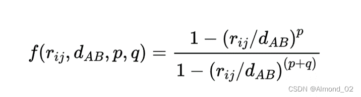
下面是两个原子之间配位数公式的表达式

 对于固定的d_AB，不同的p，q和r_ij对配位的影响，以q为横坐标，配位数f为纵坐标，下面的曲线为相应结果。下面是相应python代码。

# -*- coding: utf-8 -*-
"""
Created on Thu Feb 23 12:45:37 2023@author: sun78
"""import numpy as np
import matplotlib.pyplot as pltdef calculate_f(r_ij, d_AB, p, q):numerator = 1 - (r_ij / d_AB) ** pdenominator = 1 - (r_ij / d_AB) ** (p + q)f = numerator / denominatorreturn fplt.rcParams['figure.dpi'] = 600
# Define the range of values for q
q_values = np.linspace(1, 20, 100)# Set the values for r_ij and d_AB
r_ij = 3.5
d_AB = 2# Define the range of values for p
p_values = np.arange(1, 20)# Create a plot for all values of p
fig, ax = plt.subplots(figsize=(8, 6))
ax.set_title('Effect of q on f for different values of p')
ax.set_xlabel('q')
ax.set_ylabel('f')# Plot the results for each value of p
for p in p_values:# Calculate f for all values of q using vectorizationf_values = calculate_f(r_ij, d_AB, p, q_values)# Plot the resultsax.plot(q_values, f_values, label=f'p={p}')# Add a legend to the plot outside of the plot area
ax.legend(bbox_to_anchor=(1.05, 1), loc='upper left')plt.show()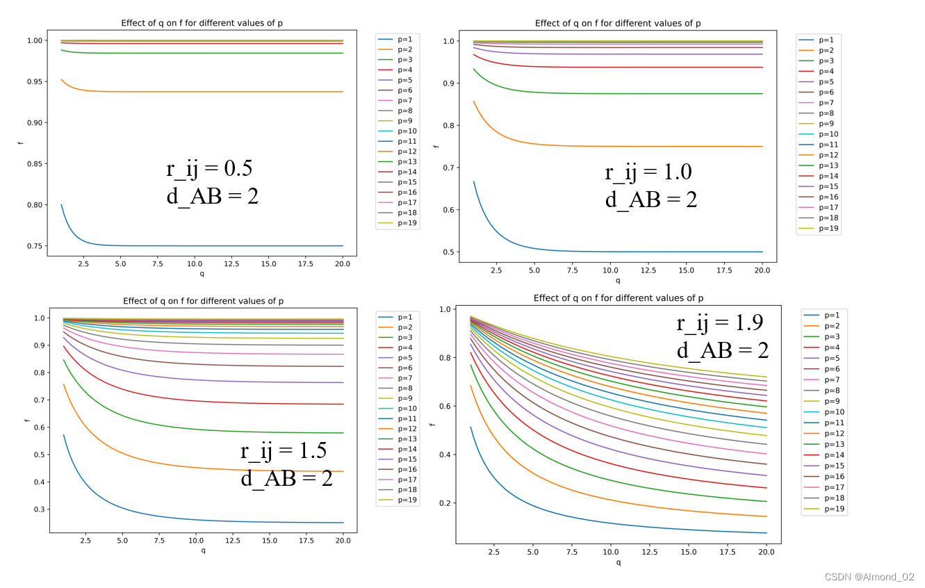

 

以r_ij为横坐标，配位数f为纵坐标，探究p，q和d_AB如何影响配位数曲线的形状

import numpy as np
import matplotlib.pyplot as pltdef calculate_f(r_ij, d_AB, p, q):numerator = 1 - (r_ij / d_AB) ** pdenominator = 1 - (r_ij / d_AB) ** (p + q)f = numerator / denominatorreturn f# Define the values of r_ij
r_values = np.linspace(0, 8, 100)# Set the values of p, q, and d_AB
p = 8
q = 6
d_AB = 2.5# Calculate f for each value of r_ij
f_values = calculate_f(r_values, d_AB, p, q)# Create a plot
fig, ax = plt.subplots(figsize=(8, 6))
ax.set_title('Effect of r_ij on f')
ax.set_xlabel('r_ij')
ax.set_ylabel('f')
ax.plot(r_values, f_values)plt.show()

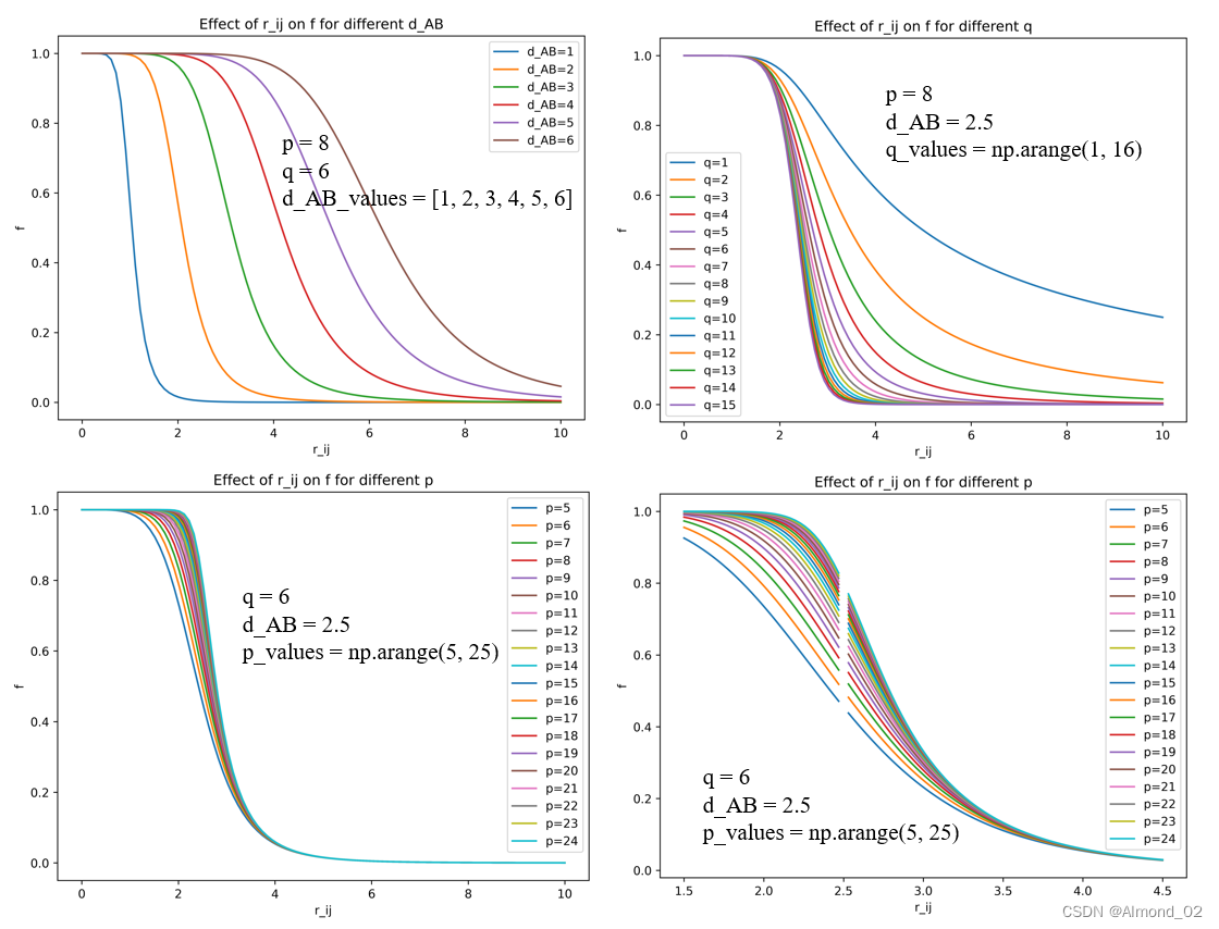
d_AB对曲线形状影响代码

import numpy as np
import matplotlib.pyplot as pltdef calculate_f(r_ij, d_AB, p, q):numerator = 1 - (r_ij / d_AB) ** pdenominator = 1 - (r_ij / d_AB) ** (p + q)f = numerator / denominatorreturn f# Define the values of r_ij
r_values = np.linspace(0, 10, 100)# Set the values of p, q, and d_AB
p = 8
q = 6
d_AB_values = [1, 2, 3, 4, 5, 6]# Calculate f for each value of r_ij and each value of d_AB
f_values = []
for d_AB in d_AB_values:f_values.append(calculate_f(r_values, d_AB, p, q))# Create a plot
fig, ax = plt.subplots(figsize=(8, 6))
ax.set_title('Effect of r_ij on f for different d_AB')
ax.set_xlabel('r_ij')
ax.set_ylabel('f')
for i, d_AB in enumerate(d_AB_values):ax.plot(r_values, f_values[i], label=f'd_AB={d_AB}')
ax.legend()plt.show()

q 对曲线形状影响代码

import numpy as np
import matplotlib.pyplot as pltdef calculate_f(r_ij, d_AB, p, q):numerator = 1 - (r_ij / d_AB) ** pdenominator = 1 - (r_ij / d_AB) ** (p + q)f = numerator / denominatorreturn f# Define the values of r_ij
r_values = np.linspace(0, 10, 100)# Set the values of p, q, and d_AB
p = 8
d_AB = 2.5
q_values = np.arange(1, 16)# Calculate f for each value of r_ij and each value of q
f_values = []
for q in q_values:f_values.append(calculate_f(r_values, d_AB, p, q))# Create a plot
fig, ax = plt.subplots(figsize=(8, 6))
ax.set_title('Effect of r_ij on f for different q')
ax.set_xlabel('r_ij')
ax.set_ylabel('f')
for i, q in enumerate(q_values):ax.plot(r_values, f_values[i], label=f'q={q}')
ax.legend()plt.show()

 p 对曲线形状影响代码

import numpy as np
import matplotlib.pyplot as pltdef calculate_f(r_ij, d_AB, p, q):numerator = 1 - (r_ij / d_AB) ** pdenominator = 1 - (r_ij / d_AB) ** (p + q)f = numerator / denominatorreturn f# Define the values of r_ij
r_values = np.linspace(0, 10, 100)# Set the values of p, q, and d_AB
q = 6
d_AB = 2.5
p_values = np.arange(5, 25)# Calculate f for each value of r_ij and each value of p
f_values = []
for p in p_values:f_values.append(calculate_f(r_values, d_AB, p, q))# Create a plot
fig, ax = plt.subplots(figsize=(8, 6))
ax.set_title('Effect of r_ij on f for different p')
ax.set_xlabel('r_ij')
ax.set_ylabel('f')
for i, p in enumerate(p_values):ax.plot(r_values, f_values[i], label=f'p={p}')
ax.legend()plt.show()

参考资料： CP2K_INPUT / MOTION / FREE_ENERGY / METADYN / METAVAR

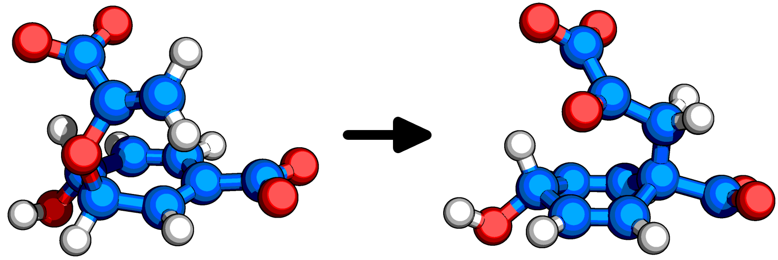
3. Biochemical systems metadynamics 

We have now simulated a full QM/MM system for 5 ps. Unfortunately, as we can see in the metadynamics logfile and in the .xyz trajectory file, no reaction occurred. This makes sense, as there is a significant energy barrier to overcome. One option would be to run this simulation for months on end, hoping for the reaction to occur spontaneously. A second, more practical option would be to bias the system. We will use metadynamics to bias our collective variables (CVs). The metadynamics procedure adds new a gaussian potential at the current location after a number of MD steps, controlled by MOTION/FREE_ENERGY/METADYN#NT_HILLS, encouraging the system to explore new regions of CV space. The height of the gaussian can be controlled with the keyword MOTION/FREE_ENERGY/METADYN#WW, while the width can be controlled with MOTION/FREE_ENERGY/METADYN/METAVAR#SCALE. These three parameters determine how the energy surface will be explored. Exploring with very wide and tall gaussians will explore various regions of your system quickly, but with poor accuracy. On the other hand, if you use tiny gaussians, it will take a very long time to fully explore your CV space. An issue to be aware of is hill surfing: when gaussians are stacked on too quickly, the simulation can be pushed along by a growing wave of hills. Choose the MOTION/FREE_ENERGY/METADYN#NT_HILLS parameter large enough to allow the simulation to equilibrate after each hill addition.

You can now run the metadynamics simulation using metadynamics.inp.

&GLOBALPROJECT METADYNPRINT_LEVEL LOWRUN_TYPE MD
&END GLOBAL&FORCE_EVALMETHOD QMMMSTRESS_TENSOR ANALYTICAL&DFTCHARGE -2&QSMETHOD AM1&SE&COULOMBCUTOFF [angstrom] 10.0&END&EXCHANGECUTOFF [angstrom] 10.0&END&END&END QS&SCFMAX_SCF 30EPS_SCF 1.0E-6SCF_GUESS ATOMIC&OTMINIMIZER DIISPRECONDITIONER FULL_SINGLE_INVERSE&END&OUTER_SCFEPS_SCF 1.0E-6MAX_SCF 10&END&PRINT&RESTART OFF&END&RESTART_HISTORY OFF&END&END&END SCF&END DFT&MM&FORCEFIELDPARMTYPE AMBERPARM_FILE_NAME complex_LJ_mod.prmtop&SPLINEEMAX_SPLINE 1.0E8RCUT_NB [angstrom] 10&END SPLINE&END FORCEFIELD&POISSON&EWALDEWALD_TYPE SPMEALPHA .40GMAX 80&END EWALD&END POISSON&END MM&SUBSYS&CELLABC [angstrom] 79.0893744057 79.0893744057 79.0893744057ALPHA_BETA_GAMMA 90 90 90&END CELL&TOPOLOGYCONN_FILE_FORMAT AMBERCONN_FILE_NAME complex_LJ_mod.prmtop&END TOPOLOGY&KIND NA+ELEMENT Na&END KIND&COLVAR&DISTANCE_FUNCTIONCOEFFICIENT -1ATOMS  5663 5675 5670 5671&END DISTANCE_FUNCTION&END COLVAR&END SUBSYS&QMMMECOUPL COULOMB&CELLABC 40 40 40ALPHA_BETA_GAMMA 90 90 90&END CELL&QM_KIND OMM_INDEX 5668 5669 5670 5682 5685 5686&END QM_KIND&QM_KIND CMM_INDEX 5663 5666 5667 5671 5673 5675 5676 5678 5680 5684&END QM_KIND&QM_KIND HMM_INDEX  5664 5665 5672 5674 5677 5679 5681 5683&END QM_KIND&END QMMM
&END FORCE_EVAL&MOTION&MDENSEMBLE NVTTIMESTEP [fs] 0.5STEPS    60000  !30000 fs = 30 psTEMPERATURE 298&THERMOSTATTYPE NOSEREGION GLOBAL&NOSETIMECON [fs] 100.&END NOSE&END THERMOSTAT&END MD&FREE_ENERGYMETHOD METADYN&METADYNDO_HILLS  .TRUE.NT_HILLS 100WW [kcalmol] 1.5&METAVARWIDTH 0.5 !Also known as scaleCOLVAR 1&END METAVAR&PRINT&COLVARCOMMON_ITERATION_LEVELS 3&EACHMD 10&END&END&END&END METADYN&END FREE_ENERGY&PRINT&RESTART                                    ! This section controls the printing of restart files&EACH                                     ! A restart file will be printed every 10000 md stepsMD 5000&END&END&RESTART_HISTORY                            ! This section controls dumping of unique restart files during the run keeping all of them.Most useful if recovery is needed at a later point.&EACH                                     ! A new restart file will be printed every 10000 md stepsMD 5000&END&END&TRAJECTORY                                 ! Thes section Controls the output of the trajectoryFORMAT XYZ                                ! Format of the output trajectory is XYZ&EACH                                     ! New trajectory frame will be printed each 100 md stepsMD 1000&END&END&END PRINT
&END MOTION&EXT_RESTARTRESTART_FILE_NAME MONITOR-1.restartRESTART_COUNTERS .FALSE.
&END

The evolution of the collective variables over time can be observed in the METADYN-COLVAR.metadynLog file. The substrate can be found near the 3 to 8 bohr CV region, whereas the product can be found near the -3 to -8 bohr region. For this tutorial, we will stop the simulation once we have sampled the forward and reverse reaction once. In a production setting you should observe several barrier crossings and observe the change in free energy profile as a function of simulation time. The free energy landscape for the reaction can be obtained by integrating all the gaussians used to bias the system. Fortunately, CP2K comes with the graph.sopt tool that does this all for you. You will need to compile this program separately if you don't have it already. Run the tool passing the restart file as input.

graph.sopt -cp2k -file METADYN-1.restart -out fes.dat

This outputs the fes.dat file, containing a one-dimensional energy landscape. Plot it to obtain a graph charting the energy as a function of the distance difference.

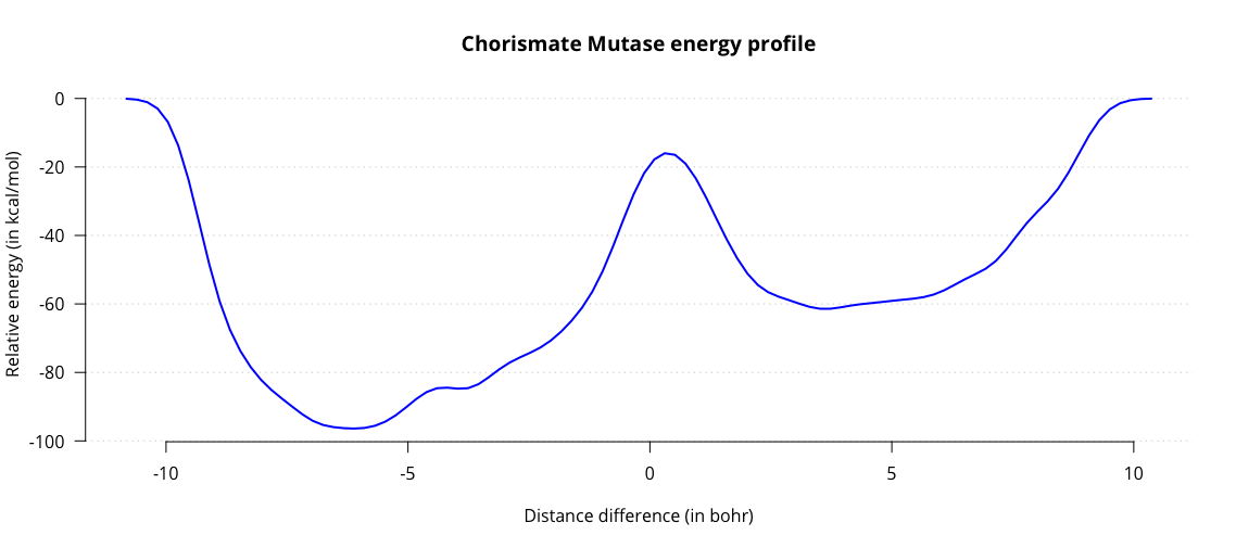
Observe the two energy minima for substrate and product, and the maximum associated with the transition state. From this graph we can estimate the activation energy in the enzyme, amounting to roughly 44 kcal/mol. Results from literature generally estimate the energy to be around 20 kcal/mol. While we are in the right order of magnitude, our estimate is not very accurate. One contributing factor might be our choice of QM/MM subsystems. Up to this point we have only treated our substrate with QM and everything else with MM. This is a significant simplification, which could affect our energy barrier.

参考资料：howto:biochem_qmmm [CP2K Open Source Molecular Dynamics ]

4. 自由能面绘图软件graph.sopt

"graph.sopt" is a tool used to visualize and analyze the output from a CP2K simulation. It is specifically designed for use with CP2K's "SOPT" optimization algorithm, which is a powerful tool for finding the global minimum energy configuration of a molecular system.

The "graph.sopt" tool can be used to visualize the energy landscape of the system, including the positions of minima, transition states, and saddle points. This information can be used to gain insight into the dynamics of the system and to understand the mechanisms of molecular transformations.

"graph.sopt" can be used with a variety of input and output file formats, including CP2K output files, XYZ files, and Gaussian output files. It provides a range of visualizations, including energy profiles, molecular animations, and 3D plots of the energy landscape.

Overall, the "graph.sopt" tool is a valuable resource for those using CP2K for molecular simulations, particularly for optimization studies. It can provide valuable insights into the behavior of molecular systems and help to understand the mechanisms of molecular transformations.

5. cp2k和plumed联用简单案例

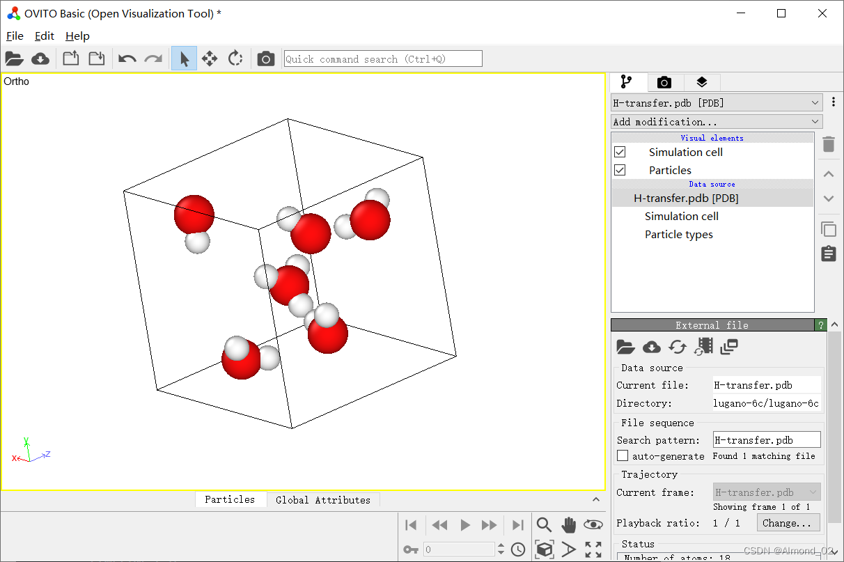
This is a molecular dynamics input file for simulating a system of water molecules using density functional theory. The simulation is performed using the NVT ensemble with a thermostat of the CSVR type. The simulation runs for 100 steps with a timestep of 1.0, and a temperature of 300 K. The force evaluation is performed using the Quickstep method with the BLYP exchange-correlation functional. The input file includes information about the cell size, topology, basis set, and potential files. The free energy calculations have been commented out.

&MOTION&MDENSEMBLE NVTSTEPS 100TIMESTEP 1.0TEMPERATURE 300.0&THERMOSTATTYPE CSVR&CSVRTIMECON 1.0&END CSVR&END THERMOSTAT&END MD
# &FREE_ENERGY
#   &METADYN
#     USE_PLUMED .TRUE.
#     PLUMED_INPUT_FILE ./plumed.dat
#   &END METADYN
# &END FREE_ENERGY
&END MOTION
&FORCE_EVALMETHOD Quickstep&DFTBASIS_SET_FILE_NAME BASIS_SETPOTENTIAL_FILE_NAME POTENTIAL&MGRIDCUTOFF 340REL_CUTOFF 50 &END MGRID&SCFEPS_SCF 1.0E-6MAX_SCF 100SCF_GUESS atomic&OTPRECONDITIONER FULL_ALLMINIMIZER DIIS&END OT&END SCF&XC&XC_FUNCTIONAL BLYP &END XC_FUNCTIONAL&END XC&PRINT&E_DENSITY_CUBE&END E_DENSITY_CUBE&END PRINT&END DFT&SUBSYS&CELLABC 7.83 7.83 7.83&END CELL&TOPOLOGYCOORD_FILE_NAME H-transfer.pdb COORD_FILE_FORMAT PDBCONN_FILE_FORMAT OFF&END TOPOLOGY&KIND OBASIS_SET DZVP-GTH-BLYP POTENTIAL GTH-BLYP-q6&END KIND&KIND HBASIS_SET DZVP-GTH-BLYP POTENTIAL GTH-BLYP-q1&END KIND&END SUBSYS
&END FORCE_EVAL
&GLOBALPROJECT waterRUN_TYPE MD PRINT_LEVEL LOW 
&END GLOBAL

参考资料：PLUMED: Lugano tutorial: Computing proton transfer in water

6. Tree diagram of keywords ralated to metadynamics

Note: The tree diagram shows the hierarchy of the sections and keywords, where the root is CP2K_INPUT, and each level represents the subsections and keywords under the parent section. 

In CP2K input file, the section that controls the run of metadynamics is the &METADYN section. This section contains several sub-sections that allow you to specify the parameters for running metadynamics, such as the height and width of the Gaussian hills, and the frequency of hill deposition. Additionally, you can specify the collective variables used in metadynamics in the &COLVAR section.

CP2K_INPUT
├── ATOM
├── DEBUG
├── EXT_RESTART
├── FARMING
├── FORCE_EVAL
├   ├── BSSE
├   ├── DFT
├   ├── EIP
├   ├── EMBED
├   ├── EXTERNAL_POTENTIAL
├   ├── MIXED
├   ├── MM
├   ├── NNP
├   ├── PRINT
├   ├── PROPERTIES
├   ├── PW_DFT
├   ├── QMMM
├   ├── RESCALE_FORCES
├   ├── SUBSYS
├   ├   ├── CELL
├   ├   ├── COLVAR
├   ├   ├   ├── ACID_HYDRONIUM_DISTANCE
├   ├   ├   ├── ACID_HYDRONIUM_SHELL
├   ├   ├   ├── ANGLE
├   ├   ├   ├── ANGLE_PLANE_PLANE
├   ├   ├   ├── BOND_ROTATION
├   ├   ├   ├── COLVAR_FUNC_INFO
├   ├   ├   ├── COMBINE_COLVAR
├   ├   ├   ├── CONDITIONED_DISTANCE
├   ├   ├   ├── COORDINATION
├   ├   ├   ├   ├── POINT
├   ├   ├   ├   ├── ATOMS_FROM
├   ├   ├   ├   ├── ATOMS_TO
├   ├   ├   ├   ├── ATOMS_TO_B
├   ├   ├   ├   ├── KINDS_FROM
├   ├   ├   ├   ├── KINDS_TO
├   ├   ├   ├   ├── KINDS_TO_B
├   ├   ├   ├   ├── ND
├   ├   ├   ├   ├── ND_B
├   ├   ├   ├   ├── NN
├   ├   ├   ├   ├── NN_B
├   ├   ├   ├   ├── R0
├   ├   ├   ├   └── R0_B
├   ├   ├   ├── DISTANCE
├   ├   ├   ├── DISTANCE_FROM_PATH
├   ├   ├   ├── DISTANCE_FUNCTION
├   ├   ├   ├── DISTANCE_POINT_PLANE
├   ├   ├   ├── GYRATION_RADIUS
├   ├   ├   ├── HBP
├   ├   ├   ├── HYDRONIUM_DISTANCE
├   ├   ├   ├── HYDRONIUM_SHELL
├   ├   ├   ├── POPULATION
├   ├   ├   ├── PRINT
├   ├   ├   ├── QPARM
├   ├   ├   ├── REACTION_PATH
├   ├   ├   ├── RING_PUCKERING
├   ├   ├   ├── RMSD
├   ├   ├   ├── TORSION
├   ├   ├   ├── U
├   ├   ├   ├── WC
├   ├   ├   ├── XYZ_DIAG
├   ├   ├   └── XYZ_OUTERDIAG
├   ├   ├── COORD
├   ├   ├── CORE_COORD
├   ├   ├── CORE_VELOCITY
├   ├   ├── KIND
├   ├   ├── MULTIPOLES
├   ├   ├── PRINT
├   ├   ├── RNG_INIT
├   ├   ├── SHELL_COORD
├   ├   ├── SHELL_VELOCITY
├   ├   ├── TOPOLOGY
├   ├   ├── VELOCITY
├   ├   └── SEED
├   ├── METHOD
├   └── STRESS_TENSOR
├── GLOBAL
├── MULTIPLE_FORCE_EVALS
├── NEGF
├── OPTIMIZE_BASIS
├── OPTIMIZE_INPUT
├── SWARM
├── TEST
├── VIBRATIONAL_ANALYSIS
└── MOTION├── BAND├── CELL_OPT├── CONSTRAINT├── DRIVER├── FLEXIBLE_PARTITIONING├── GEO_OPT├── MC├── MD├── PINT├── PRINT├── SHELL_OPT├── TMC└── FREE_ENERGY├── ALCHEMICAL_CHANGE├── FREE_ENERGY_INFO├── METADYN│ ├── EXT_LAGRANGE_FS│ ├── EXT_LAGRANGE_SS│ ├── EXT_LAGRANGE_SS0│ ├── EXT_LAGRANGE_VVP│ ├── METAVAR│ │ ├── WALL│ │ ├── COLVAR│ │ ├── GAMMA│ │ ├── LAMBDA│ │ ├── MASS│ │ └── SCALE│ ├── MULTIPLE_WALKERS│ ├── PRINT│ ├── SPAWNED_HILLS_HEIGHT│ ├── SPAWNED_HILLS_INVDT│ ├── SPAWNED_HILLS_POS│ ├── SPAWNED_HILLS_SCALE│ ├── COLVAR_AVG_TEMPERATURE_RESTART│ ├── DELTA_T│ ├── DO_HILLS│ ├── HILL_TAIL_CUTOFF│ ├── LAGRANGE│ ├── LANGEVIN│ ├── MIN_DISP│ ├── MIN_NT_HILLS│ ├── NHILLS_START_VAL│ ├── NT_HILLS            │ ├── OLD_HILL_NUMBER│ ├── OLD_HILL_STEP│ ├── PLUMED_INPUT_FILE│ ├── P_EXPONENT│ ├── Q_EXPONENT│ ├── SLOW_GROWTH│ ├── STEP_START_VAL│ ├── TAMCSTEPS│ ├── TEMPERATURE│ ├── TEMP_TOL│ ├── TIMESTEP│ ├── USE_PLUMED│ ├── WELL_TEMPERED│ ├── WTGAMMA│ └── WW└── UMBRELLA_INTEGRATION

下面是cp2k元动力学输入文件中关于&COLVAR（CP2K_INPUT / FORCE_EVAL / SUBSYS / COLVAR）和&FREE_ENERGY重要部分 。

&COLVAR&COORDINATIONKINDS_FROM  SiKINDS_TO   SiR_0 [angstrom]  2.6NN  16ND  20&END COORDINATION&END COLVAR&COLVAR&COORDINATIONKINDS_FROM  SiKINDS_TO   HR_0 [angstrom]  2.0NN  8ND  14&END COORDINATION&END COLVAR&COLVAR&COORDINATIONKINDS_FROM  HKINDS_TO    HR_0 [angstrom]  1.8NN  8ND  14&END COORDINATION&END COLVAR&FREE_ENERGY&METADYNDO_HILLS NT_HILLS 100WW 2.0e-3LAGRANGETEMPERATURE 300.TEMP_TOL  10.&METAVARLAMBDA  2.5MASS   30.SCALE 0.1COLVAR 1&END METAVAR&METAVARLAMBDA 3.0MASS 30.0SCALE 0.25COLVAR 2&END METAVAR&METAVARLAMBDA 3.0MASS 30.0SCALE 0.25COLVAR 3&WALLPOSITION 0.0TYPE QUARTIC&QUARTICDIRECTION WALL_MINUSK  100.0&END&END&END METAVAR&PRINT&COLVARCOMMON_ITERATION_LEVELS 3&EACHMD 1&END&END&HILLSCOMMON_ITERATION_LEVELS 3&EACHMD 1&END&END&END&END METADYN&END

Here are some of the main keywords in CP2K related to metadynamics:

WW: Specifies the height of the gaussian to spawn.

"SCALE" is a keyword under the METAVAR section which is used to specify the scaling factors for the collective variables. The expression WW * Sum_{j=1}^{nhills} Prod_{k=1}^{ncolvar} [EXP[-0.5*((ss-ss0(k,j))/SCALE(k))^2]] for this term includes a Gaussian function with a width controlled by the SCALE factor.

Specifies the scale factor for the following collective variable. The history dependent term has the expression: WW * Sum_{j=1}^{nhills} Prod_{k=1}^{ncolvar} [EXP[-0.5*((ss-ss0(k,j))/SCALE(k))^2]], where ncolvar is the number of defined METAVAR and nhills is the number of spawned hills.

"COLVAR" is another keyword under the METAVAR section, which is used to specify the collective variables themselves. A collective variable is a function of the atomic coordinates that describes some aspect of the system's behavior. For example, the distance between two atoms, the angle between three atoms, or the RMSD of a protein structure are all examples of collective variables that could be used in a metadynamics simulation.

NT_HILLS：Specify the maximum MD step interval between spawning two hills. When negative, no new hills are spawned and only the hills read from SPAWNED_HILLS_* are in effect. The latteris useful when one wants to add a custom constant bias potential.

In CP2K, the NT_HILLS keyword is used to specify the maximum MD step interval between spawning two hills in a metadynamics simulation. This parameter controls the rate at which new Gaussian hills are added to the bias potential, which helps to explore the free energy surface of the system being studied.

When the value of NT_HILLS is positive, a new Gaussian hill is spawned at every NT_HILLS time steps, and the maximum number of spawned hills is determined by the value set for NT_HILLS in the &METADYNAMICS section.

When the value of NT_HILLS is negative, no new hills are spawned during the simulation, and only the hills that have already been deposited are taken into account. This can be useful when one wants to apply a custom constant bias potential, as the hills that have already been deposited can provide a rough approximation of the free energy surface, which can be combined with a constant bias potential to generate a more accurate representation of the system's behavior.

WALL: In CP2K, the "MATAVAR" section is used to define the variables that will be biased during a metadynamics simulation, and the "WALL" keyword is an option that can be used to define a hard wall on the bias potential. When a hard wall is used, the bias potential is set to a very large value when the variable reaches a certain value, effectively preventing the system from exploring those regions of the potential energy surface.

DO_HILLS: DO_HILLS是一个逻辑类型的关键字，用于控制是否生成Hills。默认值为.FAlSE.，即不生成Hills。这个关键字只能使用一次，接受一个逻辑值。该关键字可以被视为一个开关，将其设为.lTRUE.可以打开生成Hills的功能。

The DO_HILLS keyword is used in metadynamics simulations to control the generation of Gaussian hills, which are used to bias the system away from free energy minima and explore a wider range of conformational space. When set to .TRUE., the keyword enables the spawning of Gaussian hills, while setting it to .FALSE. disables the generation of hills. This keyword allows users to control the timing and duration of hill spawning during a metadynamics simulation.

In summary, when NT_HILLS is positive, new hills are spawned at regular intervals, and when it is negative, no new hills are spawned, and only the deposited hills are used in the simulation.

7. CP2K元动力学中获取重构势能面的方法

跑完cp2k的metadynamics后，获取的最重要的文件包括轨迹文件，COLVAR.metadynLog文件，以及restart文件，restart文件可以被用于构建重构的自由能面，需要利用cp2k编译时自带的软件，叫做graph.sopt。

通过graph.sopt对于restart文件的处理，我们会获得一个叫做fes.dat的文件，该文件前几列是集体变量，最后一列是能量的值，这些参数都采用原子单位制，比如长度单位使用bohr，能量单位使用哈特里（Hartree），我们需要将长度单位换算成埃，并考虑盒子的周期性，将能量单位换算成KJ/mol。

1 bohr = 0.52917721067 Å

1 Hartree = 2625.4996 kJ/mol

获得了单位换算后的fes.dat数据后，可以利用gnuplot或者python来绘制重构的二位自由能面。

How to reconstruct the free energy surface in metadynamics using cp2k？

To reconstruct the free energy surface in metadynamics using CP2K, you need to use a post-processing tool called fes.sopt, which is available in the CP2K/tools/fes directory . This tool can read the restart file of CP2K, which contains the information of the bias potential and the collective variables, and calculate the free energy surface by subtracting the bias potential from the total potential. You can use the following command to run the fes.sopt tool:

fes.sopt -cp2k -ndim 3 -ndw 1 2 3 -file <FILENAME>.restart

where -cp2k indicates that the input file is from CP2K, -ndim 3 indicates that there are three collective variables, -ndw 1 2 3 indicates that the first, second and third collective variables are used to calculate the free energy surface, and -file <FILENAME>.restart indicates the name of the restart file. You will get a fes.dat file that contains the 3D free energy surface .

You can also use other options to control the output format, the grid size, the smoothing algorithm, and the re-weighting method. You can use fes.sopt -h to see the help information. You can also use manual.cp2k.org to find more information about the fes.sopt tool and the metadynamics section in CP2K. I hope this helps. 

注意：fes.dat文件中，最后一列为自由能，单位是a.u.，前面几列为CV。绘图时一般采用kJ/mol，注意换算。

参考资料：

CP2K软件metadynamics模块的自由能后处理问题 - 第一性原理 (First Principle) - 计算化学公社

8. 基于restart文件继续执行元动力学

You can use the restart file of cp2k to continue the metadynamics by adding the section `EXT_RESTART` to your input file and setting `RESTART_METADYNAMICS` to `.TRUE.`. You also need to specify the name of the restart file with `FILENAME` keyword.

For example, if your restart file is named `metadyn.restart`, you can add something like this to your input file:

&EXT_RESTARTFILENAME metadyn.restartRESTART_METADYNAMICS .TRUE.
&END EXT_RESTART

另外一个例子

&EXT_RESTARTRESTART_FILE_NAME  si6_clu_mtd_l_p2-1.restartRESTART_COUNTERS   TRESTART_POS        TRESTART_VEL        TRESTART_THERMOSTAT TRESTART_METADYNAMICS T
&END EXT_RESTART

下面是EXT_RESTART小节下的一些典型关键词，该小节下的所有关键词都默认为TRUE，所以其实只需要把RESTART_FILE_NAME关键词写上就可以了。

EXT_RESTART	Section for external restart, specifies an external input file where to take positions, etc. By default they are all set to TRUE
RESTART_COUNTERS	Restarts the counters in MD schemes and optimization STEP The lone keyword behaves as a switch to .TRUE.
RESTART_POS	Takes the positions from the external file The lone keyword behaves as a switch to .TRUE.
RESTART_VEL	Takes the velocities from the external file The lone keyword behaves as a switch to .TRUE.
RESTART_THERMOSTAT	Restarts the nose thermostats of the particles from the EXTERNAL file The lone keyword behaves as a switch to .TRUE.
RESTART_METADYNAMICS	Restarts hills from a previous metadynamics run from the EXTERNAL file The lone keyword behaves as a switch to .TRUE.
RESTART_FILE_NAME	Specifies the name of restart file (or any other input file) to be read. Only fields relevant to a restart will be used (unless switched off with the keywords in this section)  Alias names for this keyword: EXTERNAL_FILE

参考资料

How to do a restart in cp2k — pwtools documentation

9. 元动力学测试题

here's a multiple choice test for middle level learners on metadynamics:

1 What is metadynamics in molecular dynamics simulations?
a) A method to simulate chemical reactions in a solvent
b) A method to enhance sampling of rare events
c) A method to visualize molecular structures
d) A method to study the electronic properties of molecules

2 What is the goal of metadynamics in molecular dynamics simulations?
a) To minimize the energy of the system
b) To maximize the energy of the system
c) To enhance the sampling of the free energy landscape
d) To prevent the system from evolving

3 How does the metadynamics bias potential evolve during a simulation?
a) It remains constant throughout the simulation
b) It decreases during the simulation
c) It increases during the simulation
d) It evolves dynamically to enhance sampling

4 What is the difference between well-tempered metadynamics and standard metadynamics?
a) Well-tempered metadynamics uses a higher temperature than standard metadynamics
b) Well-tempered metadynamics uses a lower temperature than standard metadynamics
c) Well-tempered metadynamics uses a modified bias potential to enhance sampling
d) Well-tempered metadynamics uses a different collective variable than standard metadynamics

5 What is the role of the collective variables in metadynamics simulations?
a) To define the atoms in the system
b) To define the force field used in the simulation
c) To define the reaction coordinates of the system
d) To define the sampling frequency of the simulation

6 What is the relationship between the height of the bias potential and the frequency of the sampling of the CV space?
a) Higher bias potential leads to lower sampling frequency
b) Higher bias potential leads to higher sampling frequency
c) Lower bias potential leads to lower sampling frequency
d) Lower bias potential leads to higher sampling frequency

7 How can one determine the optimal Gaussian width for a metadynamics simulation?
a) By trial and error
b) By using a fixed width that works for all simulations
c) By using a narrow width to enhance sampling
d) By using a wider width to enhance sampling

8 What is the role of the hill-climbing algorithm in metadynamics simulations?
a) To optimize the collective variables
b) To optimize the bias potential
c) To optimize the force field
d) To optimize the temperature

9 What is the difference between on-the-fly and post-processing analysis of metadynamics simulations?
a) On-the-fly analysis is faster than post-processing analysis
b) On-the-fly analysis is more accurate than post-processing analysis
c) On-the-fly analysis is performed during the simulation, while post-processing analysis is performed after the simulation
d) On-the-fly analysis is performed after the simulation, while post-processing analysis is performed during the simulation

10 What are some of the advantages of using metadynamics in molecular dynamics simulations?
a) Enhanced sampling of rare events
b) Accurate prediction of thermodynamic properties
c) Fast convergence to the equilibrium state
d) All of the above

Answers:

1. b
2. c
3. d
4. c
5. c
6. a
7. a
8. b
9. c
10. d

结论：chatGPT总是会输出一些cp2k中并不存在的关键词，关键词的逻辑顺序有时候也会出错，对关键词地解释目前也存在较大偏差，目前的帮助还很非常有限。

参考资料：

howto:biochem_qmmm [CP2K Open Source Molecular Dynamics ]

PLUMED: Lugano tutorial: Computing proton transfer in water